Schroedinger's equation for the eigenstates of one particle in one dimension is HY(x)=EY(x), where H is the Hamiltonian operator. For a particle subject to a potential V(x) and using atomic units, H is -0.5*d^2/dx^2+V(x). Schroedinger's equation may be solved to yield a set of eigenvalues, Ei and the corresponding eigenfunctions, Yi(x). These are the allowed energies of the system and the probability amplitude of the particle at each position. The probability of finding the particle at a certain position is the square of Y(x). Y(x) is normalized, so that the integral of Y(x)^2dx over all x is 1.
The following discussion will use "bra-ket" notation. The expression [A|B|C] is defined to be the integral over all x of A B C dx. Usually, A and C are wavefunctions, and B is an operator.
Exact solutions of Schroedinger's equations only exist for a few simple V(x). Numerical solutions may be obtained by representing Y(x) as a linear combination of a finite set of basis functions,Pi(x). This converts the problem into a matrix equation, HC=ENC, where C is a vector of coefficients, H is a matrix whose elements Hji=[Pj|H|Pi], and N is a matrix whose elements Nji=[Pj|1|Pi]. Often, the Pi are chosen to be orthogonal, so that N=I.
Another approach is suitable for finding the smallest eigenvalue and eigenstate. The energy of any Y(x) can be evaluated at E=[Y|H|Y]/[Y|1|Y]. Starting from any initial Y(x) and minimizing E will approach the actual ground state energy, E0, and eigenstate Y0. Since this is just another way of solving the eigenvalue problem, it will converge well. For this project, I have chosen the minimization approach, since it is simpler and should be faster at finding the ground state.
The Y(x) will be represented as cubic Bsplines with N evenly spaced knots. Bsplines were chosen initially to satisfy the course requirements, but they turn out to have many desirable properties. Since the basis is local, evaluation of the E integrals takes only constant order time. If V(x) is also represented as a cubic bspline with the same knots, all the integrals in E can be solved analytically at low cost. Since E involves an integral of a second derivative of Y, it is nice to have Y be at least once differentiable. If Y were, for example, piecewise linear, all the curvature would be concentrated at the knots instead of spread evenly. This would suggest using quadratic b-splines, but I had more familiarity with cubic b-splines.
The algorithm is as follows. Choose a cubic Bspline representation of the potential function V(x). In addition to this V(x), the potential is taken to be infinite outside the range 0 to W. This is equivalent to constraining Y(0)=0 and Y(W)=0. Choose initial deBoor points for Y(x). The boundary constraints are met by adding two additional deBoor points on each side. Finally, do conjugate gradient descent on E.
The code consists of three modules, psi.c, draw.c, and fit.c which include psi.h Psi.c contains code to evaluate the integrals in E and the derivative of E with respect to the deBoor points of Y. It also contains the main command line interface. Draw.c simply draws Bsplines to a text file suitable for plotting with gnuplot. Fit.c contains energy and gradient computations for doing a least-squares fit of a Bspline to a user defined potential function.
Four of my libraries are used. List.c provides variable length array support, with searching and sorting. Recalc.c is a subminimal recalc engine, which allows a program to create and then evaluate variables with formulae. Vector.c provides n-dimensional vector operations. Minimize.c does conjugate gradient descent.
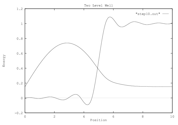
Three V(x) functions were tried. The first was a "box" potential, with V(x)=0 in the range 0 to 10 and infinite outside. The second was a harmonic potential, V(x)=0.08*(x-10)^2 from 0 to 20 and infinite outside. The third was a two level well, V(x)=0 from 0 to 5 and V(x)=1 from 5 to 10 and infinite outside 0 to 10. The first two have analytic solutions, and the shape, although not the exact energy can be found for the third.
The box potential ground state is one half a sine wave. Y(x)=sqrt(2/W)*sin(pi*x/W) and E0=(pi/W)^2/2. For W=10, E0=0.04934802200544679309. The analytic and numerical solutions for this V(X) are shown in Box Well for a 10 knot Bspline. The match is very close between the analytic and numerical solution, even though only 10 deBoor points were used. The potential V(X) is also graphed, and by convention, the Y(x) is offset by its energy.
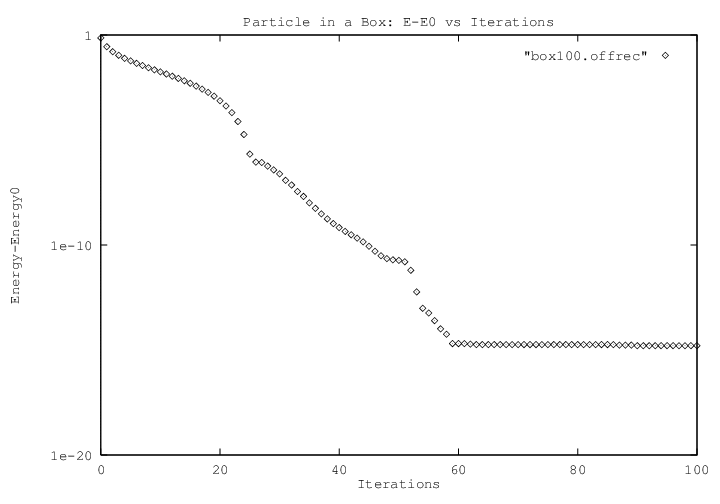
The convergence toward E0 versus number of iterations is shown in Box Well: E vs Time for a 100 knot Bspline. At the end of the run, the numerical solution agrees in energy with the analytic to 13 significant figures. As usual, the convergence is exponential.
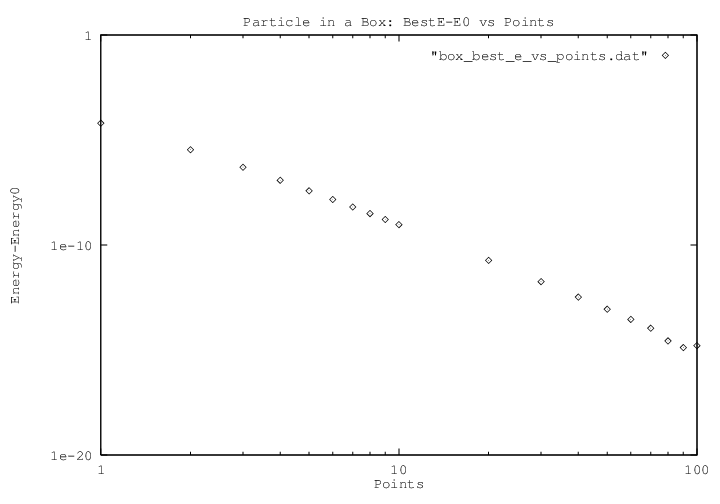
Even when the numerical solution has converged to its final answer, it will still have an energy higher than the exact solution, because the cubic bspline cannot precisely represent a sine wave. This remaining error is shown in Box Well: BestE vs Points for various numbers of knots. The relationship appears to be polynomial, error=b*iterations^a, with a=-5.64, This number gives me no insight.
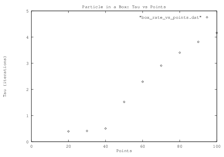
Finally, the characteristic time constant of the exponential convergence is compared in Box Well: Tau vs Points for various numbers of knots. Although the data is noisy for smaller numbers of knots, it appears to be linear in N. This is exactly as expected for conjugate gradient descent on a near-parabolic energy function. Considering that each iteration also takes O(N), the overall time of convergence is O(N^2).
The solution of the harmonic potential is E0=0.2 and Y(x)=(2*E0/pi)^0.25*e^(-E0*x^2). In the numerical solution, the infinite potential outside 0 and 20 does not substantially effect the result, since the probability density near the boundaries is already negligible. Also, the cubic bspline for the potential can faithfully represent a quadratic, so no major error is added here. The analytic and numerical solutions for this V(x) are shown in Harmonic Well for a 10 knot Bspline. Here the curves don't match as well, since many of the evenly spaced knots are in regions of little interest. Of course, more deBoor points will generate a much better fit.
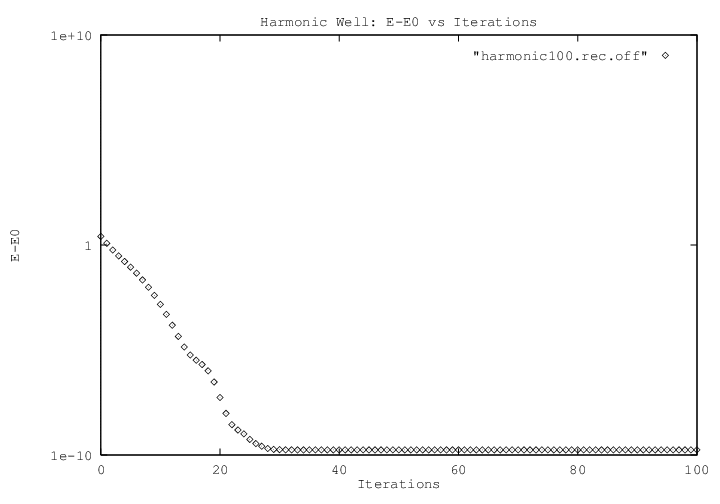
The convergence toward E0 is shown in Harmonic Well: E vs Time for a 100 knot Bspline. The convergence is exponential. The final energy agrees to 9 significant figures with the analytic solution.
The best energy versus number of points is shown in Harmonic Well: BestE vs Points. Note that for small numbers of points, the odd numbers are favored. After a while, though, the best energy is again polynomial in the number of points.
The two level well is a sine wave from 0 to 5 and a decaying exponential from 5 to 10. They meet at x=5 with matching slopes. Solving this constraint involves a transcendental equation, so the energy can't be computed analytically. A numerical solution is shown in Two Level Well for 10 knots. The most notable feature is that the step is not fit very well by a cubic bspline with 10 knots. It does demonstrate that the least squares curve fitting is working.
Cubic Bsplines are an excellent basis to find quantum ground states. The locality and polynomial form of the wavefunction and potential function make evaluating the energy or its gradient a simple linear time operation, without the need for approximate numerical integration. The convergence time is O(N^2), where N is the number of independent variables.
The next step is the extend the program to 3 dimensions and many particles. The wavefunction exists in 3P dimensional space, where P is the number of particles. It can be represented as a 3P dimensional cubic tensor product B-spline surface. The potential is 3 dimensional. The Pauli exclusion principle requires that the wavefunction be antisymmetric under the exchange of two particles coordinates. This reduces the interesting domain by P!. Making the deBoor points antisymmetric will guarantee that the function is too. Aside from these small changes, the algorithm will still work.
Another possible improvement might be to convert to a piecewise cubic wavelet basis. This might improve the order of convergence. However, the wavefunction already has long distance information transfer via the normalization. The condition number of the problem is probably very good already. More significantly, an adaptive refinement algorithm would be a major improvement, especially over 3P dimensional space.